Intro
This dashboard covers the course materials for the course Markup Languages and Reproducible Programming in Statistics

Instructor: Gerko Vink
Study load: 2.5 ECTS
Assessment: Final Assignment
Course folder
| When? | Where? | |
|---|---|---|
| 14-Sep | 9 am | Ruppert 011 |
| 28-Sep | 9 am | Ruppert 011 |
| 02-Nov | 9 am | Ruppert 011 |
| 09-Nov | 9 am | Ruppert 011 |
| 23-Nov | 9 am | Ruppert 011 |
| 07-Dec | 9 am | Ruppert 011 |
Quick Overview
Column 1
This course gives an overview of the state-of-the-art in statistical markup, reproducible programming and scientific digital representation. Students will get to know the professional field of statistical markup and its innovations and challenges. It consists of 6 meetings in which students will learn about markup languages (( and Markdown), learn efficient and reproducible programming with rMarkdown, experience developing Shiny web apps, get to know version control with Git and will create and maintain their own data archive repository and personal (business card) page through GitHub. Combining these lectures, the students get acquainted with different viewpoints on marking up statistical manuscripts, areas of innovation, and challenges that people face when working with, analysing and reporting (simulated) data. Knowledge obtained from this course will help students face multidimensional problems during their professional career.
Assignment and Grading
The final grade is computed as follows
| Graded part | Weight |
|---|---|
| Markup manuscript | 50 % |
| Research repository | 40 % |
| Personal repository | 10 % |
To develop the necessary skills for completing the assignment and the presentation, 6 exercises must be made and submitted. These exercises are not graded, but students must fulfill them to pass the course.
In order to pass the course, the final grade must be 5.5 or higher, your contribution to the course should be sufficient and all assignments and practical assignments should be handed in and/or passed. Otherwise, additional work is required concerning the assignments and/or exercises you have failed.
Column 2
Schedule
| When? | Where? | What? | |
|---|---|---|---|
| 14-Sep | 9 am | Ruppert 011 | Monte Carlo simulation and Git |
| 28-Sep | 9 am | Ruppert 011 | Reproducible workflows and replication |
| 02-Nov | 9 am | Ruppert 011 | Typesetting equations with LaTeX |
| 09-Nov | 9 am | Ruppert 011 | Version control and Github in depth |
| 23-Nov | 9 am | Ruppert 011 | Presentations with rMarkdown |
| 07-Dec | 9 am | Ruppert 011 | Github pages and Shiny |
For fun
Expand \((a+b)^n\): \[ \begin{gather*} (a + b)^n\\ (a\ + \ b)^n\\ (a\quad + \quad b)^n\\ (a\qquad + \qquad b)^n \end{gather*} \] source
Course Manual
Column 1
Course manual
Course description
This course gives an overview of the state-of-the-art in statistical markup, reproducible programming and scientific digital representation. Students will get to know the professional field of statistical markup and its innovations and challenges. It consists of 6 meetings in which students will learn about markup languages (LaTeX and Markdown), learn efficient and reproducible programming with rMarkdown, experience developing Shiny web apps, get to know version control with Git and will create and maintain their own data archive repository and personal (business card) page through GitHub. Combining these lectures, the students get acquainted with different viewpoints on marking up statistical manuscripts, areas of innovation, and challenges that people face when working with, analysing and reporting (simulated) data. Knowledge obtained from this course will help students face multidimensional problems during their professional career.
Assignment
Students will individually choose one statistical topic and work on a manuscript about this topic. Students will need to perform calculations and program code for this manuscript. All work for the student needs to be combined in an easy understandable and insightful data archive and will need be posted on a personal GitHub repository. This end result will be graded on 1) Quality of the markup language skills, 2) Quality of the data archive and 3) Quality of the online repository.
Grading
Students will be evaluated on the following aspects:
- Developing and publishing a research archive that contains code, data and a typeset manuscript following a markup language;
- Developing and publishing a research archive that demonstrate a reproducible workflow.
- Developing and publishing a personal repository page;
- Students develop fundamental knowledge and understanding in the state of the art in statistical markup languages and reproducible programming (Knowledge and Understanding)
- They apply their knowledge in a multi-disciplinary context to contemporary problems (Applying)
- They can determine the most effective markup strategies to address a typesetting problem (Applying)
- They can efficiently organise a reproducible programming process (Applying)
- They can advise researchers in applying the current state of the art in markup and programming (Judgment)
- They can produce reproducible repositories up to the standards of international programming and coding conventions and initiatives (Communication)
- They can produce publications up to the typesetting standards of international peer- reviewed journals (Communication)
- They are capable of autonomous scholarly self-development (Learning skills)
- They give proof of being a responsible and scholarly professional (Learning skills)
After taking this course students can understand innovations in statistical markup, statistical simulation and reproducible research. Students are also able to approach challenges from different professional viewpoints. They have gained experience in marking up a professional manuscript and designing a state-of-the-art statistical archive in an open source repository.
Grading
To develop the necessary skills for completing the assignment and the presentation, 6 exercises must be made and submitted. These exercises are not graded, but students must fulfil them to pass the course.
The final grade is computed as follows
| Graded part | Weight |
|---|---|
| Markup manuscript | 50 % |
| Research repository | 40 % |
| Personal repository | 10 % |
In order to pass the course, the final grade must be 5.5 or higher, your contribution to the course should be sufficient and all assignments and practical assignments should be handed in and/or passed. Otherwise, additional work is required concerning the assignments and/or exercises you have failed.
Literature
Relevant documents that are used in the course and/or may provide useful additional reading will be placed on or referred to on the course website.
Instructions for preparing the repositories
The research repository has to be prepared as a supplementary archive that can serve as an extensive documentation of the research (e.g. as a supplement to be submitted to a journal). The archive has to be published in a public or private GitHub repository.
Time schedule
This course takes place in the first semester. The course will run over 6 meetings (Wednesdays 9-12am) during the semester, with the first meeting on September 14, 2022.
Prerequisites
Students will need their own laptop computer. Students should have experience in programming with R and should be familiar with the IDE RStudio.
Week 1
Column 1
Monte Carlo simulation and replication
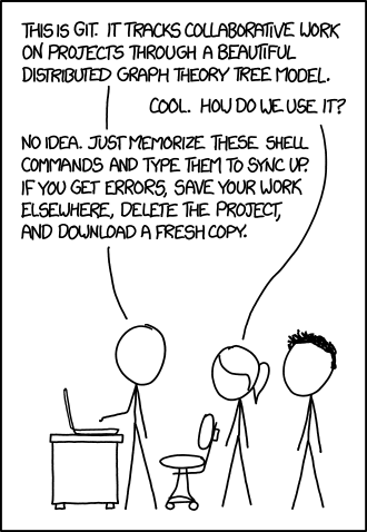
We start the hard way with Git, GitHub and
Monte Carlo simulation. Just as with any new skill aimed at
programming and/or scripting: practice makes perfect. Follow the two
exercises for this week and you’ll have a head start on the rest
of the course of your career.
All the best,
Gerko
Supplementary materials and links
The following links are very useful:
An old video walkthrough about
GitandRstudioGitHub Glossary for all terminology
this online
Gitbook is a very good resourceThis book covers pretty much everything you need to marry
gitandR.
I highly appreciate the clip on MC simulation by Ben Lambert (LEFT) and the quite comprehensive exploration of the origin and concepts of probability that govern Monte Carlo simulations by John Guttag (RIGHT).
Column 2
Slides, reading and viewing
- Slides Week 1
- Read Excuse me, do you have a moment to talk about version control? by Jennifer Bryan.
- Watch the following clip where Linus Torvalds explains that he
merely created
Gitto manage his other project
- Read this
blog post on MC simulation where Will Kurt details some quick
examples of MC simulation in
R - Then read this blog post where Will Kurt bridges the parallel to Bayesian stats
Exercises
The exercise for this week:
Week 2
Column 1
Reproducible workflows
This week we’ll cover reproducible workflows with rmarkdown in RStudio
You can find the lecture here
All the best,
For real
Please watch the below videos
Supplementary materials and links
The following links are very useful:
- RStudio’s
‘Getting Started’ with
rmarkdown - An example archive
- A comprehensive but lengthy! report aimed at avoiding and overcoming interpretation errors, non-replication, non-reproduction and fraud across science and science communication.
Column 2
Exercise and lecture
This week’s documents:
- Lecture Wk2
- Pipes make you code so much easier to interpret. Read this chapter by Hadley Wickham on pipes.
- Exercise.html
- Exercise.Rmd
- My solution to the exercise
in
Rmd - My solution to the exercise
in
html
Week 3
Column 1
Beamer and equations
This week we’ll cover equations in LaTeX - I’m sure
you’ll love it. In order to put it to the test, we will also use
LaTeX to design slide show presentations. Later on in this
course, we’ll focus on creating presentation with Markdown - which is
much easier, but also less flexible in obtaining perfect detailed
typesetting. For now, getting to know the basics of typesetting and
equations in LaTeX will pay off in the future.
All the best,
For real
Mathematicians and physicists have been using LaTeX typesetting language to craft equations in manuscripts, but now other scientists are using it too. Here’s how to get started. https://t.co/AzFaehdNXf
— Nature (@nature) October 7, 2019
Column 2
Exercise
This week’s excercise:
Supplementary materials and links
The following links are very useful for this week’s exercise:

Week 4
Column 1
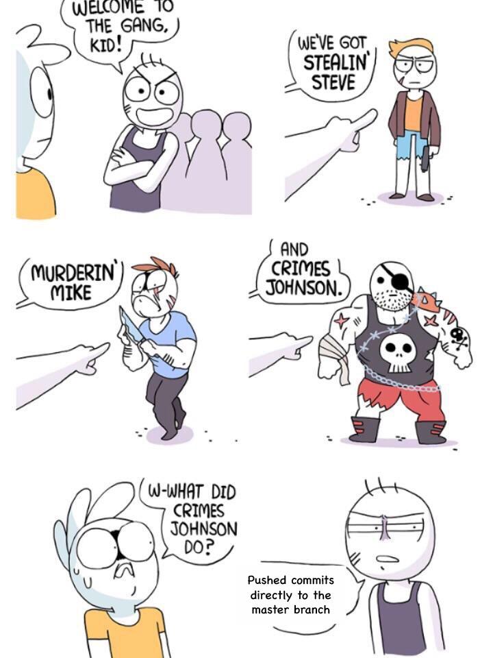
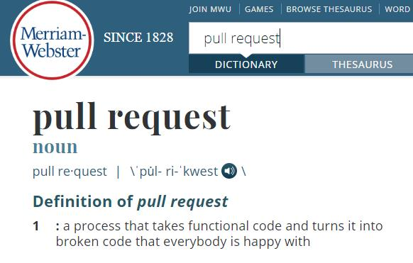
git in more detail.
This week we’ll cover git commands and procedures for
when the proverbial shit hits the fan.
All the best,

Column 2
Exercise
This week’s exercise is straightforward. Follow my lead and you’ll
learn a great deal about git
Useful links
The info in these links will take you beyond the exercise
Also
These links cover vital information about placement, sizing, etc of figures and tables and referencing. I’ll dive into it in more detail next meeting, but please study these documents links to prepare yourself.
- All background You do not have to consider the \(\LaTeX\) code per se –> just make sure that you identify the difference in look, placement and sizing of relevant components.
- Referencing
in \(\LaTeX\). This is useful
because we can use the same techniques in
markdown. All relevant materials can be found in the 2019 Archive for Week 1.
Week 5
Column 1
Presentations with rmarkdown
This week we’ll cover presentations with rmarkdown in RStudio
You can find the slides here.
All the best,
Supplementary materials and links
The following links are very useful:
Column 2
Week 6
Column 1
Online representation
This week we’ll cover shiny web-apps and
GitHub pages. shiny is a wonderful means to
showcase your work and offer online services; Hanne Oberman will share
with you her expertise. GitHub pages is the way for
developers and professionals to introduce yourself to the world and host
a personal webpage right from your GitHub. And all this is
free!
All the best,
Useful references
Definitely look at the book Mastering Shiny by Hadley Wickham. This book is currently under development.
GitHub pages
I suggest that you watch this video before you make the exercise:
Archive
Column 1
Past
Please find a sufficiently different past iteration of this course here
Deliverables
Column 1
Markup Manuscript
Your markup manuscript may be anything, but be aware that it is must be gradeable. We do not grade your manuscript on content and theoretical soundness, but will assess the visual and organizational aspects of your manuscript. Your markup manuscript must prove that you can produce a publication up to the typesetting standards of international peer-reviewed journals. So include equations, tables, figures, references, etcetera.
Research Repository
You should develop and publish a research archive that demonstrates a reproducible workflow. The archive should contain code, data and (if applicable) the typeset markup manuscript detailed above. Examples of research archives are:
Personal Repository
You should showcase yourself in a personal website, a well-covered quarto or rmarkdown document, a thoroughly designed CV. Examples are:
How to hand in your deliverables
Send us (Hanne & Gerko) an e-mail with either
- 3 links if your deliverables are online (e.g. github or some cloud service). One link for each deliverable
- 1 zip folder with 3 subfolders that contain the respective deliverables
- an email to set up an appointment to view your deliverables if it is all supersecret or private (e.g CBS data, Patient data, etc)
- any combination of the above, for any reason you deem valid. As long as it details the why and how we can(not) obtain your deliverables.
How to deal with non-CRAN code
If it is a package on GitHub, then you can easily install that with thedevtools package. For example, the following line of code
would install from my GitHub repo the mice package from
respectively the main branch and from branch estimice.
devtools::install_github("gerkovink/mice")
devtools::install_github("gerkovink/mice@estimice")
If it is not a package, but rather a series of scripts that is needed
for your research archive, you can simply load()
[workspaces] or source() [scripts] the url()
in R. For example,
load(url("https://www.gerkovink.com/yourdata.RData"))Alternatively, given that the author has allowed you to do so, you can also download the code and add it to your archive with e.g. a header and readme that indicate where you’ve obtained the source code. If you alter any code for which the source is GNU GPL v3 licences, your source needs to be open too if you intend to share it.