Synthetic data generation with mice

Gerko Vink

Thom Volker

Methodology & Statistics @ Utrecht University

November 4, 2022

Outline

• Vocabulary
• Statistical inference
• Uncertainty
• Being wrong may help
• Hello, dark data
• Embrace the darkness
• Synthetic data generation
• What should synthetic data be?

Materials

All materials can be found at

www.gerkovink.com/syn

Disclaimer

I owe a debt of gratitude to many people as the thoughts and teachings in my slides are the process of years-long development cycles and discussions with my team, friends, colleagues and peers. When someone has contributed to the content of the slides, I have credited their authorship.

When external figures and other sources are shown:

1. the references are included when the origin is known, or
2. the objects are directly linked from within the public domain and the source can be obtained by right-clicking the objects.

Scientific references are in the footer.

Opinions are my own.



Packages used:

library(mice)
library(dplyr)
library(magrittr)
library(purrr)
set.seed(123)

Vocabulary

Terms I may use

• TDGM: True data generating model
• DGP: Data generating process, closely related to the TDGM, but with all the wacky additional uncertainty
• Truth: The comparative truth that we are interested in
• Bias: The distance to the comparative truth
• Variance: When not everything is the same
• Estimate: Something that we calculate or guess
• Estimand: The thing we aim to estimate and guess
• Population: That larger entity without sampling variance
• Sample: The smaller thing with sampling variance
• Incomplete: There exists a more complete version, but we don’t have it
• Observed: What we have
• Unobserved: What we would also like to have

Statistical inference

At the start

We begin today with an exploration into statistical inference.

Statistical inference is the process of drawing conclusions from truths

Truths are boring, but they are convenient.

• however, for most problems truths require a lot of calculations, tallying or a complete census.
• therefore, a proxy of the truth is in most cases sufficient
• An example for such a proxy is a sample
• Samples are widely used and have been for a long time¹

1. See Jelke Bethlehem’s CBS discussion paper for an overview of the history of sampling within survey

Being wrong about the truth

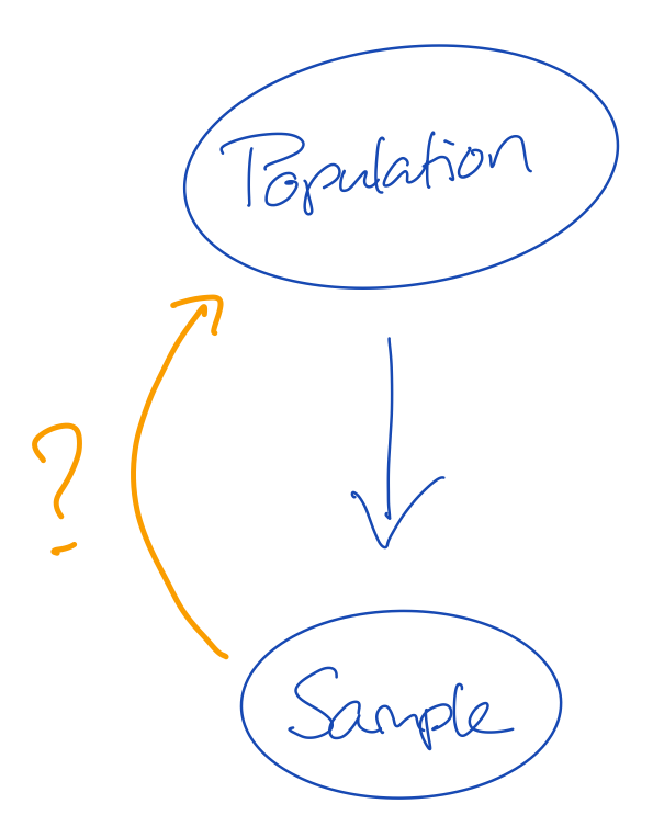
• The population is the truth
• The sample comes from the population, but is generally smaller in size
• This means that not all cases from the population can be in our sample
• If not all information from the population is in the sample, then our sample may be wrong
  
  
  Q1: Why is it important that our sample is not wrong?
  Q2: How do we know that our sample is not wrong?

Solving the missingness problem

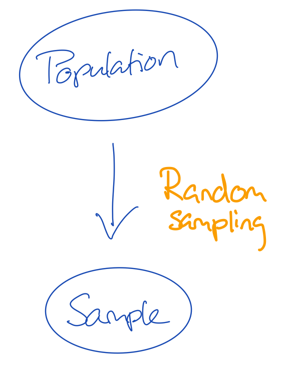
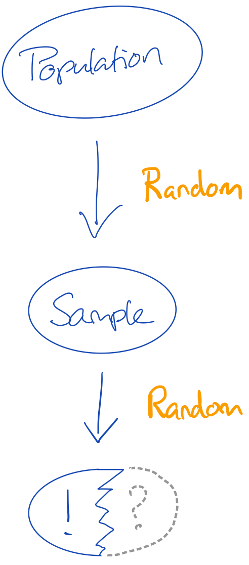
• There are many flavours of sampling
• If we give every unit in the population the same probability to be sampled, we do random sampling
• The convenience with random sampling is that the missingness problem can be ignored
• The missingness problem would in this case be: not every unit in the population has been observed in the sample

Q3: Would that mean that if we simply observe every potential unit, we would be unbiased about the truth?

Sidestep

• The problem is a bit larger

• We have three entities at play, here:

  1. The truth we’re interested in
  2. The proxy that we have (e.g. sample)
  3. The model that we’re running

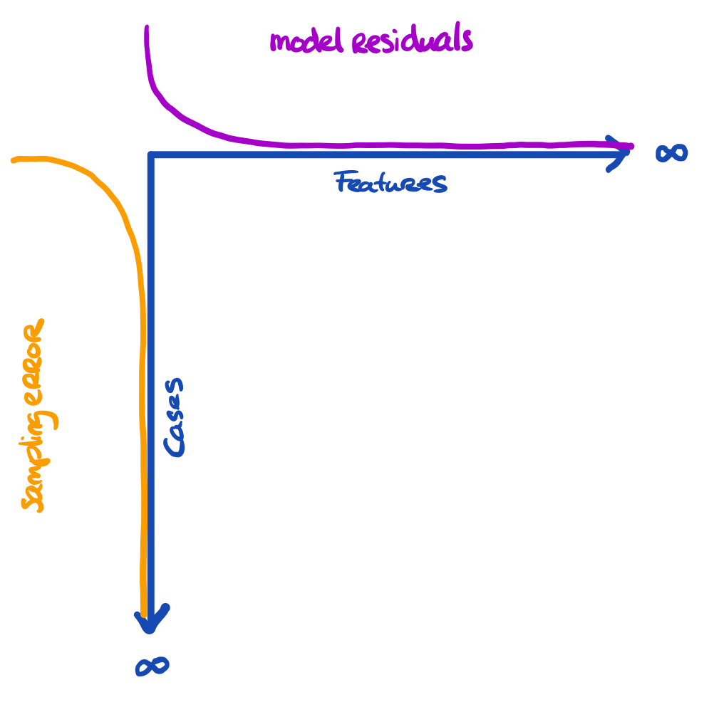
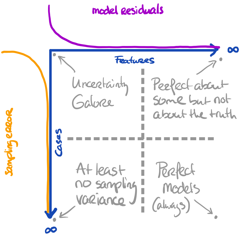
• The more features we use, the more we capture about the outcome for the cases in the data

Sidestep

• The more cases we have, the more we approach the true information

All these things are related to uncertainty. Our model can still yield biased results when fitted to \(\infty\) features. Our inference can still be wrong when obtained on \(\infty\) cases.

Sidestep

Core assumption: all observations are bonafide

Uncertainty

Uncertainty simplified

When we do not have all information:

1. We need to accept that we are probably wrong
2. We just have to quantify how wrong we are

In some cases we estimate that we are only a bit wrong. In other cases we estimate that we could be very wrong. This is the purpose of testing.

The uncertainty measures about our estimates can be used to create intervals

Confidence intervals

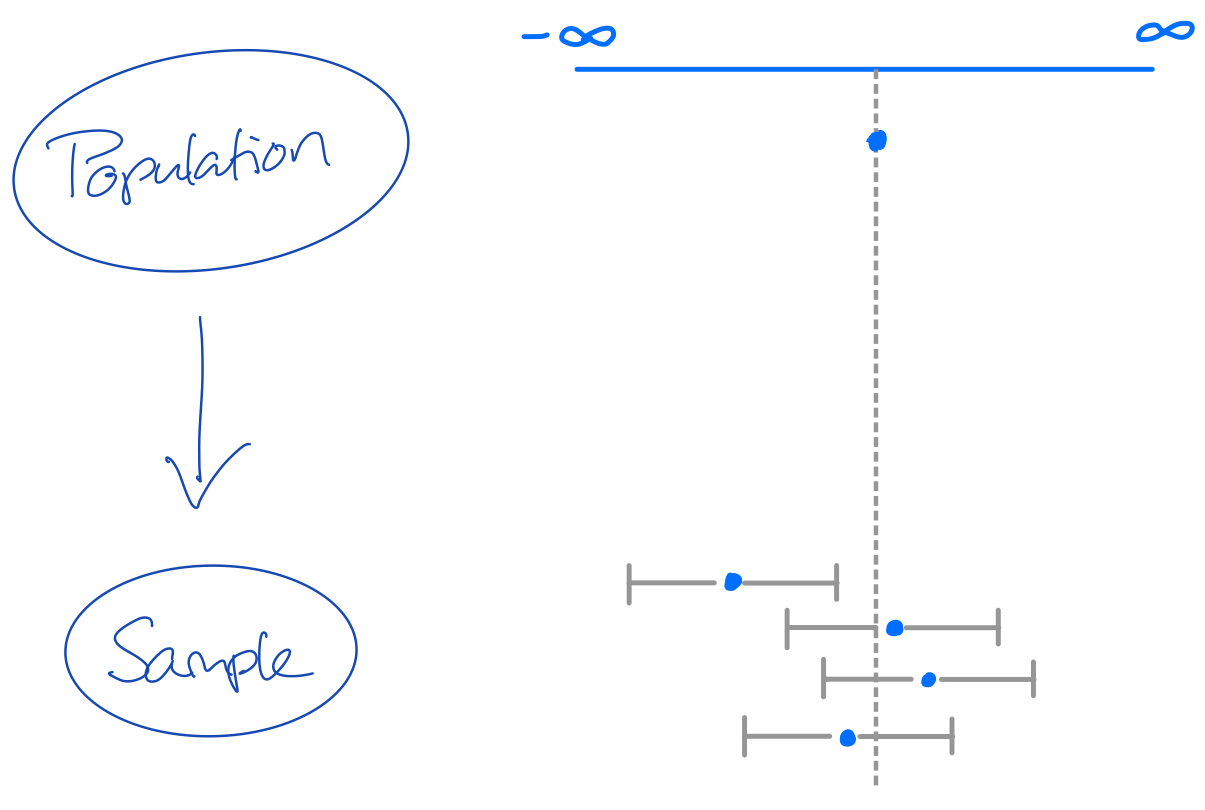
Confidence intervals can be hugely informative!

If we sample 100 samples from a population, then a 95% CI will cover the population value at least 95 out of 100 times.

• If the coverage \(<95\): bad estimation process with risk of errors and invalid inference

• If the coverage \(\geq 95\): inefficient estimation process, but correct conclusions and valid inference. Lower statistical power.

Being wrong may help

The holy trinity

Whenever I evaluate something, I tend to look at three things:

• bias (how far from the truth)
• uncertainty/variance (how wide is my interval)
• coverage (how often do I cover the truth with my interval)

As a function of model complexity in specific modeling efforts, these components play a role in the bias/variance tradeoff

Hello, dark data

Let’s do it again with missingness

We now have a new problem:

• we do not have the whole truth; but merely a sample of the truth
• we do not even have the whole sample, but merely a sample of the sample of the truth.

Q4. What would be a simple solution to allowing for valid inferences on the incomplete sample?
Q5. Would that solution work in practice?

Let’s do it again with missingness

We now have a new problem:

• we do not have the whole truth; but merely a sample of the truth
• we do not even have the whole sample, but merely a sample of the sample of the truth.

Q4. What would be a simple solution to allowing for valid inferences on the incomplete sample?
Q5. Would that solution work in practice?

Multiple imputation

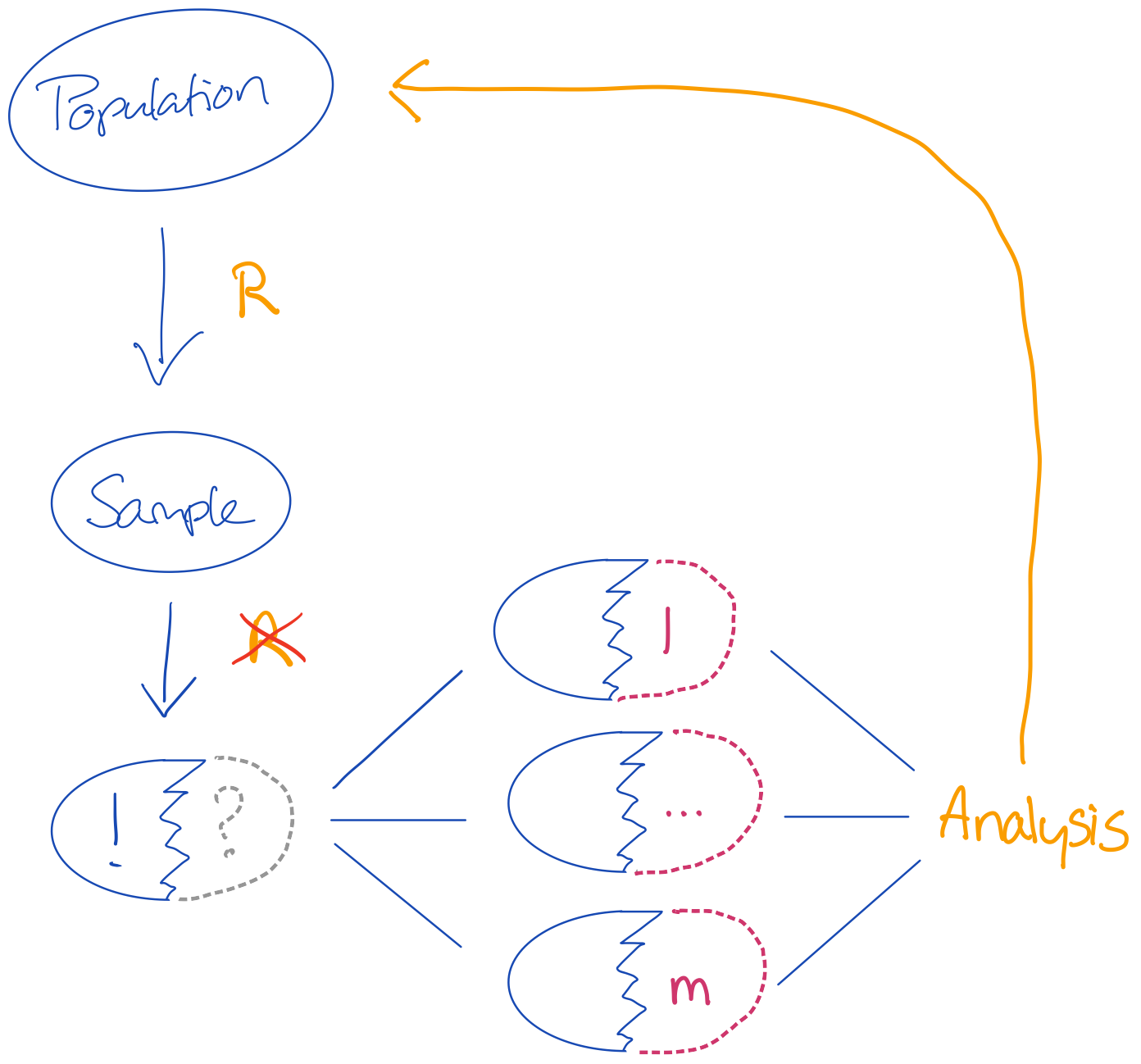
There are two sources of uncertainty that we need to cover:

1. Uncertainty about the missing value:
   when we don’t know what the true observed value should be, we must create a distribution of values with proper variance (uncertainty).
2. Uncertainty about the sampling:
   nothing can guarantee that our sample is the one true sample. So it is reasonable to assume that the parameters obtained on our sample are biased.

More challenging if the sample does not randomly come from the population or if the feature set is too limited to solve for the substantive model of interest

Embrace the darkness

Now how do we know we did well?

I’m really sorry, but:

We don’t. In practice we may often lack the necessary comparative truths!

For example:

1. Predict a future response, but we only have the past
2. Analyzing incomplete data without a reference about the truth
3. Estimate the effect between two things that can never occur together
4. Mixing bonafide observations with bonafide non-observations

What is the goal of multiple imputation?

The goal:

• IS NOT to find the correct value for a missing data point
• IS to find an answer to the analysis problem, given that there are (many) data points missing.

We are not interested in whether the imputed value corresponds to its true counterpart in the population, but we rather sample plausible values that could have been from the posterior predictive distribution

Demonstration of imputation

Let our analysis model be

boys %$% 
  lm(hgt ~ age + tv)

with output

Call:
lm(formula = hgt ~ age + tv)

Residuals:
    Min      1Q  Median      3Q     Max 
-24.679  -5.134  -0.398   5.175  23.778 

Coefficients:
            Estimate Std. Error t value Pr(>|t|)    
(Intercept) 105.4823     3.4704  30.395  < 2e-16 ***
age           3.8430     0.3262  11.782  < 2e-16 ***
tv            0.4919     0.1278   3.849 0.000155 ***
---
Signif. codes:  0 '***' 0.001 '**' 0.01 '*' 0.05 '.' 0.1 ' ' 1

Residual standard error: 8.389 on 221 degrees of freedom
  (524 observations deleted due to missingness)
Multiple R-squared:  0.7742,    Adjusted R-squared:  0.7721 
F-statistic: 378.8 on 2 and 221 DF,  p-value: < 2.2e-16

generated on 224 cases. The full data size is

[1] 748   9

Demonstration of imputation

To impute and analyze the same model with mice, we can simply run:

boys %>% 
  mice(m = 5, method = "cart", printFlag = FALSE) %>% 
  complete("all") %>% 
  map(~.x %$% lm(hgt ~ age + tv)) %>% 
  pool() %>% 
  summary()

         term   estimate  std.error  statistic        df      p.value
1 (Intercept) 71.4996462 0.62149605 115.044409 735.07926 0.000000e+00
2         age  6.9612293 0.09409268  73.982690  78.04537 0.000000e+00
3          tv -0.4650875 0.08986812  -5.175222  49.56070 4.126098e-06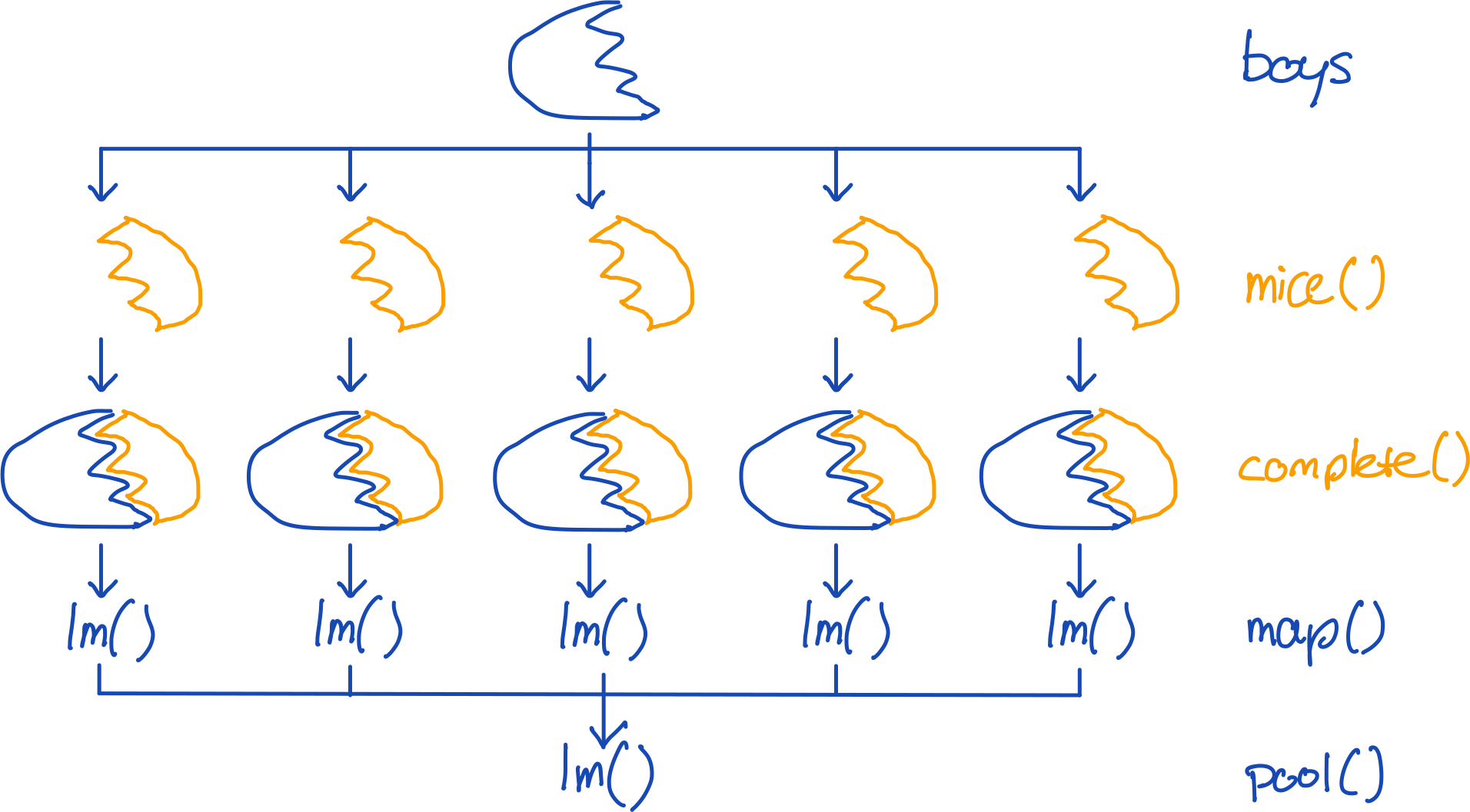

What have we done?

We have used mice to obtain draws from a posterior predictive distribution of the missing data, conditional on the observed data.

The imputed values are mimicking the sampling variation and can be used to infer about the underlying TDGM, if and only if:

• The observed data holds the information about the missing data (MAR/MCAR)

Synthetic data generation

Imputation vs Synthetisation

Instead of drawing only imputations from the posterior predictive distribution, we might as well overimpute the observed data.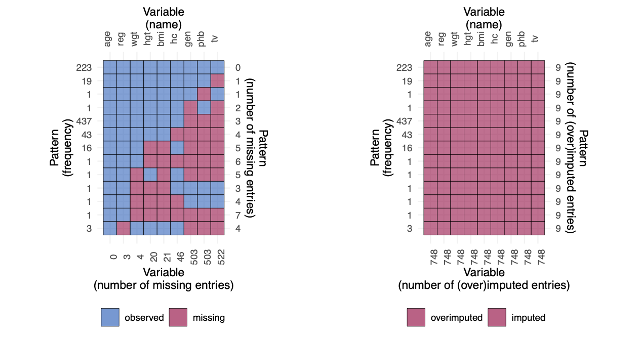

How to draw synthetic data sets with mice

boys %>% 
  mice(m = 5, method = "cart", printFlag = FALSE, where = matrix(TRUE, 748, 9)) %>% 
  complete("all") %>% 
  map(~.x %$% lm(hgt ~ age + tv)) %>% 
  pool() %>% 
  summary()

         term   estimate std.error statistic       df      p.value
1 (Intercept) 71.1914095 0.7962174 89.412020 43.37485 0.000000e+00
2         age  6.9914529 0.1141189 61.264648 45.55541 0.000000e+00
3          tv -0.4684145 0.1018189 -4.600469 42.92353 3.713106e-05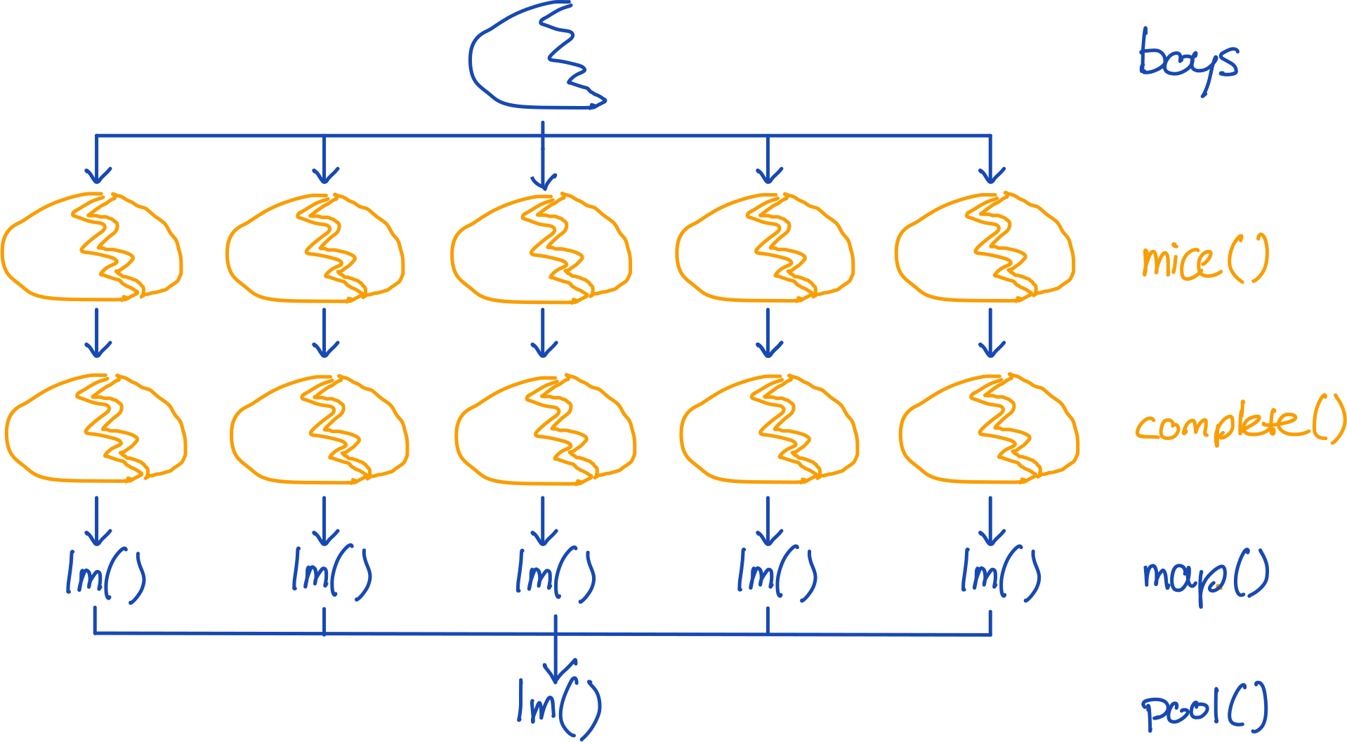

But we make an error!

Pooling in imputation

Rubin (1987, p76) defined the following rules:

For any number of multiple imputations \(m\), the combination of the analysis results for any estimate \(\hat{Q}\) of estimand \(Q\) with corresponding variance \(U\), can be done in terms of the average of the \(m\) complete-data estimates

\[\bar{Q} = \sum_{l=1}^{m}\hat{Q}_l / m,\]

and the corresponding average of the \(m\) complete data variances

\[\bar{U} = \sum_{l=1}^{m}{U}_l / m.\]

Pooling in imputation

Simply using \(\bar{Q}\) and \(\bar{U}_m\) to obtain our inferences would be to simplistic. In that case we would ignore any possible variation between the separate \(\hat{Q}_l\) and the fact that we only generate a finite set of imputations \(m\). Rubin (1987, p. 76) established that the total variance \(T\) of \((Q-\bar{Q})\) would equal

\[T = \bar{U} + B + B/m,\]

Where the between imputation variance \(B\) is defined as

\[B = \sum_{l=1}^{m}(\hat{Q}_l - \bar{Q})^\prime(\hat{Q}_l - \bar{Q}) / (m-1)\]

This assumes that some of the data are observed and remain constant over the synthetic sets

The total variance \(T\) of \((Q-\bar{Q})\) should (Reiter, 2003) equal

\[T = \bar{U} + B/m.\]

So, the correct code is

boys %>% 
  mice(m = 5, method = "cart", printFlag = FALSE, where = matrix(TRUE, 748, 9)) %>% 
  complete("all") %>% 
  map(~.x %$% lm(hgt ~ age + tv)) %>% 
  pool(rule = "reiter2003") %>% 
  summary()

         term   estimate  std.error  statistic       df      p.value
1 (Intercept) 71.1914095 0.69301891 102.726504  976.576 0.000000e+00
2         age  6.9914529 0.09973928  70.097285 1046.453 0.000000e+00
3          tv -0.4684145 0.08854244  -5.290283  962.247 1.512358e-07

Why multiple synthetic sets?

Thank back about the goal of statistical inference: we want to go back to the true data generating model.

1. We do so by reverse engineering the true data generating process
2. Based on our observed data
3. We do not know this process; hence multiple synthetic values

The multiplicity of the solution allows for smoothing over any Monte Carlo error that may arise from generating a single set.

Generating more synthetic data

mira <- boys %>% 
  mice(m = 6, method = "cart", printFlag = FALSE, where = matrix(TRUE, 748, 9)) %>% 
  list('1' = rbind(complete(., 1), complete(., 2)),
       '2' = rbind(complete(., 3), complete(., 4)),
       '3' = rbind(complete(., 5), complete(., 6))) %>% .[-1] %>% 
  data.table::setattr("class", c("mild", class(.))) %>% 
  map(~.x %$% lm(hgt ~ reg))

mira %>% pool(rule = "reiter2003") %>% 
  summary() %>% tibble::column_to_rownames("term") %>% round(3)

            estimate std.error statistic     df p.value
(Intercept)  150.427     4.684    32.114 11.731   0.000
regeast      -16.851     6.601    -2.553  6.622   0.040
regwest      -22.263     4.787    -4.650 32.970   0.000
regsouth     -23.700     5.410    -4.381 14.367   0.001
regcity      -24.295     6.477    -3.751 15.545   0.002

mira %>% pool(rule = "reiter2003", 
              custom.t = ".data$ubar * 2 + .data$b / .data$m") %>% 
  summary() %>% tibble::column_to_rownames("term") %>% round(3)

            estimate std.error statistic     df p.value
(Intercept)  150.427     5.901    25.492 11.731   0.000
regeast      -16.851     7.949    -2.120  6.622   0.074
regwest      -22.263     6.340    -3.512 32.970   0.001
regsouth     -23.700     6.901    -3.434 14.367   0.004
regcity      -24.295     8.297    -2.928 15.545   0.010

Some adjustment to the pooling rules is neede to avoid p-inflation.

Some care is needed

With synthetic data generation and synthetic data implementation come some risks.

Any idea?

What should synthetic data be?

Testing validity

Nowadays many synthetic data cowboys claim that they can generate synthetic data that looks like the real data that served as input.

This is like going to Madam Tusseaud’s: at face value it looks identical, but when experienced in real life it’s just not the same as the living thing.

Many of these synthetic data packages only focus on marginal or conditional distributions. With mice we also consider the inferential properties of the synthetic data.

In general, we argue [^4] that any synthetic data generation procedure should

1. Preserve marginal distributions
2. Preserve conditional distribution
3. Yield valid inference
4. Yield synthetic data that are indistinguishable from the real data

Example from simulation

When valid synthetic data are generated, the variance of the estimates is correct, such that the confidence intervals cover the population (i.e. true) value sufficiently [^5]. Take e.g. the following proportional odds model from Volker & Vink (2021):

term	estimate	synthetic bias	synthetic cov
age	0.461	0.002	0.939
hc	-0.188	-0.004	0.945
regeast	-0.339	0.092	0.957
regwest	0.486	-0.122	0.944
regsouth	0.646	-0.152	0.943
regcity	-0.069	0.001	0.972
G1\(|\)G2	-6.322	-0.254	0.946
G2\(|\)G3	-4.501	-0.246	0.945
G3\(|\)G4	-3.842	-0.244	0.948
G4\(|\)G5	-2.639	-0.253	0.947

End of presentation

A. Bacall