library(mice)     # for imputation and amputation
library(purrr)    # for functional programming
library(furrr)    # for functional futures
library(mvtnorm)  # for multivariate normal data
library(magrittr) # for pipes
library(dplyr)    # for data manipulation
library(tibble) # for tibblesStrategies for simulating missingness
All quarto files and R-code to reproduce this document can be found in this repository on GitHub.
Aim
The aim of this document is to outline several strategies for simulation missingness that allow for valid inferences. Such simulation scenarios would evaluate the following multiple imputation pipeline:

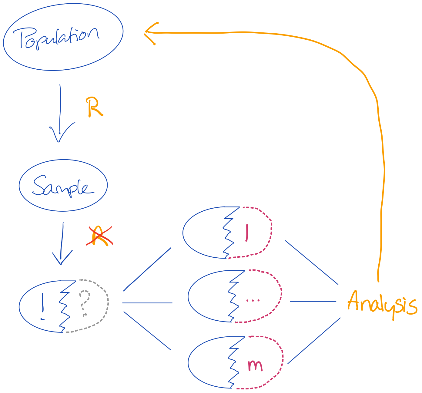
Figure 1: A standard imputation workflow
In the above workflow a sample is randomly obtained from a truth (e.g. a population). This sample may be nonrandomly missing, which means that the imputation procedure must correct the inference for its combined analysis to allow for valid conclusions about the population.
I will focus on three types of methods for evaluating imputation procedures: model-based simulation, design-based simulation and methods that depart from the above workflow by merely generating a single finite set wherein only missingness is induced.
Analysis model
The analysis model is a simple linear regression model. In all simulation scenarios I will use 3 variables/features: an outcome \(y\) and 2 predictors \(x\) and \(z\), such that
\[y = x + z + \varepsilon,\]
where the residual \(\varepsilon\sim\mathcal{N}(0, 1)\).
I will evaluate the analysis model on the imputed data and on the complete cases in order to demonstrate the effect of the missingness.
Missingness generation
All missingness will be simulated with the ampute() function (Schouten, Lugtig, and Vink 2018) from package mice (Van Buuren and Groothuis-Oudshoorn 2011). To illustrate the simluation approaches, I will induce missingness according to an MCAR (Rubin 1976) and right-tailed MAR (Schouten and Vink 2021) mechanism.
R packages
I use the following packages in this document
The references for these packages are respectively: Van Buuren and Groothuis-Oudshoorn (2011), Henry and Wickham (2022), Vaughan and Dancho (2022), Genz et al. (2021), Bache and Wickham (2022), Wickham et al. (2022) and Müller and Wickham (2022).
I also fix the RNG seed to allow for full reproduction of the findings:
set.seed(123) # get the same as I gotModel-based simulation
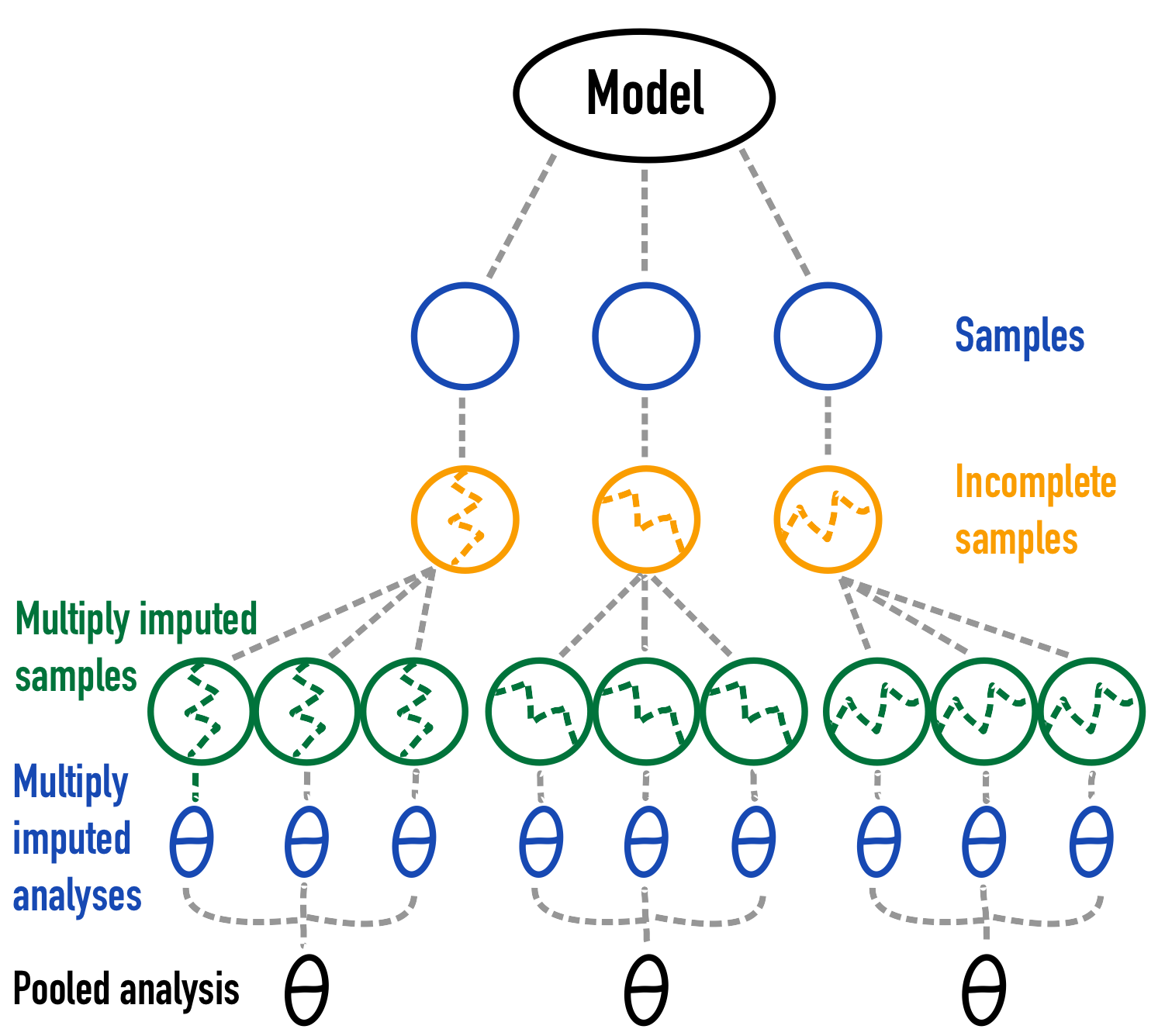
The first strategy I outline is model-based simulation, where a theoretical model is used to sample the data from. The estimand - or true parameter - will be the parameter value in the theoretical population where I sample from. The below figure outlines this approach.

Figure 2: A graphical depiction of model based simulation 1.
Let’s keep it simple and use a multivariate normal model to sample our data from. In this case, we generate a predictor space \((x,z)\) by drawing data from a multivariate normal distribution with means
\[ \mu = \begin{pmatrix} 8 \\ 3 \end{pmatrix}, \] and variance-covariance matrix
\[
\Sigma =
\begin{pmatrix}
1 & .2 \\
.2 & 1
\end{pmatrix}.
\] Let’s generate the simulation data by drawing a predictor space from a multivariate normal distribution with package mvtnorm (Genz et al. 2021) in R (R Core Team 2022). I also add the outcome \(y\) following
\[y = 6x + 3z + \varepsilon, \]
where \(\varepsilon = \mathcal{N}(0, 1)\). The following code realizes this:
sigma <- matrix(data = c(1, 0.7, 0.7, 1),
                ncol = 2)
simdata <- replicate(n = 1000,
                     expr = mvtnorm::rmvnorm(n = 1000,
                                             mean = c(8, 3),
                                             sigma = sigma) %>%
                       as_tibble() %>% # make into a tibble
                       rename(x = V1, z = V2) %>% # rename columns
                       mutate(y = 6 * x + 3 * z + rnorm(1000)), # add y
                     simplify = FALSE) # keep as list of generated sets
Warning: The `x` argument of `as_tibble.matrix()` must have unique column names if
`.name_repair` is omitted as of tibble 2.0.0.
ℹ Using compatibility `.name_repair`.The simdata object is a list with 1000 sampled data sets. For every data set there is an \(y\), an \(x\) and a \(z\) variable.
simdata[[1]] %>% # the first simulated set
  head()
# A tibble: 6 × 3
x z y
<dbl> <dbl> <dbl>
1 7.39 2.58 51.6
2 9.47 3.65 68.0
3 8.77 4.64 66.0
4 7.95 2.00 54.9
5 7.20 2.33 50.3
6 9.27 3.80 66.4We’d expect that the data would approximate \(y = 6x + 3z\) as the data are generated that way. But, since we are simulating, we can verify:
simdata %>%
  map(~.x %$% # for every simulated set in simdata....
        lm(y ~ x + z) %>% # fit linear model
        coefficients) %>% # extract coefficients
  Reduce("+", .) / length(simdata) # add all and divide by length (= average)
(Intercept) x z
-0.008753601 6.001663721 2.998499808 We see indeed that the average simulated set approximates the true parameters for the \(Intercept\), for \(x\) and for \(z\).
Simulate MCAR missingness
Now, let’s use a future to set up the amputation and imputation in a computationally efficient manner. We’ll start with the MCAR simulation:
mbased_MCAR <-
  simdata %>%
  furrr::future_map(function(x) {
    x %>%
      ampute(prop = .5,
             mech = "MCAR") %>% .$amp %>%
      mice(m = 5,
           maxit = 5,
           method = "norm",
           print = F)
  }, .options = furrr_options(seed = 123))
The object mbased_MCAR is a list where each listed element is a multiply imputed data set (mice class mids).
mbased_MCAR[[1]]Class: mids
Number of multiple imputations: 5
Imputation methods:
x z y
"norm" "norm" "norm"
PredictorMatrix:
x z y
x 0 1 1
z 1 0 1
y 1 1 0All mids objects contain the incomplete ata, so there is no need to store that seperately. It can easily be extracted from the mids object, e.g.:
mbased_MCAR[[1]]$data %>%
  head()
x z y
1 7.394101 NA 51.57804
2 9.469680 NA 68.01869
3 8.768088 4.636654 65.97690
4 7.948440 2.003083 54.91912
5 7.195638 2.327744 50.33119
6 9.269263 3.795884 NAA simple evaluation of the analysis model would demonstrate that the results are unbiased under MCAR:
mbased_MCAR %>%
  map(~.x %>% # for every simulated multiple imputation....
        complete("all") %>% # create a list of completed data sets
        map(~.x %$% # for every completed data set....
              lm(y ~ x + z)) %>% # fit linear model
              pool() %>%  # pool coefficients
              summary(conf.int = TRUE) %>% # summary of coefficients
              mutate(true = c(0, 6, 3), # add true
                     cov = `2.5 %` < true & true < `97.5 %`, # coverage
                     bias = estimate - true) %>% # bias
              column_to_rownames("term")) %>% # `term` as rownames
      Reduce("+", .) / length(mbased_MCAR) # add all and divide by length
estimate std.error statistic df p.value
(Intercept) -0.02353421 0.38784260 -0.06524533 39.45521 4.978151e-01
x 6.00425139 0.06105269 100.93209692 44.71173 2.147031e-11
z 2.99699882 0.06118896 50.29176172 42.83921 1.048865e-09
2.5 % 97.5 % true cov bias
(Intercept) -0.8473295 0.8002611 0 0.940 -0.023534210
x 5.8747674 6.1337354 6 0.937 0.004251391
z 2.8671356 3.1268620 3 0.939 -0.003001178The results demonstrate that the estimates are unbiased and confidence valid cf. Neyman (1934).
Simulate MAR missingness
We can easily replicate the above example for a right-tailed MAR mechanism by adapting the following code changes to the simulation:
mbased_MAR <-
  simdata %>%
  furrr::future_map(function(x) {
    x %>%
      ampute(prop = .5,
             mech = "MAR", type = "RIGHT") %>% .$amp %>%
      mice(m = 5,
           maxit = 5,
           method = "norm",
           print = F)
  }, .options = furrr_options(seed = 123))
and to the evaluation:
mbased_MAR %>%
  map(~.x %>% # for every simulated multiple imputation....
        complete("all") %>% # create a list of completed data sets
        map(~.x %$% # for every completed data set....
              lm(y ~ x + z)) %>% # fit linear model
              pool() %>%  # pool coefficients
              summary(conf.int = TRUE) %>% # summary of coefficients
              mutate(true = c(0, 6, 3), # add true
                     cov = `2.5 %` < true & true < `97.5 %`, # coverage
                     bias = estimate - true) %>% # bias
              column_to_rownames("term")) %>% # `term` as rownames
      Reduce("+", .) / length(mbased_MCAR) # add all and divide by length
estimate std.error statistic df p.value 2.5 %
(Intercept) 0.009213976 0.39579355 0.02031572 45.45269 4.801810e-01 -0.8382059
x 5.999835575 0.06293355 98.28587904 44.12498 3.287930e-11 5.8649385
z 2.996801955 0.06225600 49.49150216 40.66474 7.306357e-10 2.8639024
97.5 % true cov bias
(Intercept) 0.8566338 0 0.933 0.0092139760
x 6.1347326 6 0.936 -0.0001644251
z 3.1297015 3 0.955 -0.0031980455Design-based simulation
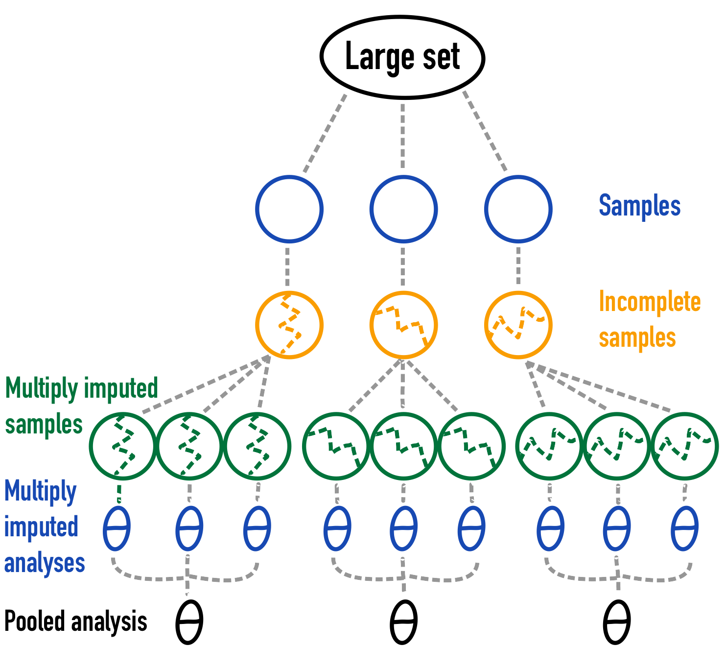
With design-based simulation, a smaller set is usually sampled from a sufficiently large finite register or finite population. This type of simulation design is often deployed when a real-life data source is available, such as in e.g. medical or official statistics.

Figure 3: A graphical depiction of design-based simulation2.
Generating a sufficiently large set
We continue with the previously used multivariate normal model, but now sample a true set of size 1,000,000 cases. The easiest and most computationally convenient approach to realizing this, would be to bind the 1000 sets from simdata together into a long format:
truth <- simdata %>%
  do.call("rbind", .)
The resulting object truth is a 1000000 by 3 tibble.
truth # A tibble: 1,000,000 × 3
x z y
<dbl> <dbl> <dbl>
1 7.39 2.58 51.6
2 9.47 3.65 68.0
3 8.77 4.64 66.0
4 7.95 2.00 54.9
5 7.20 2.33 50.3
6 9.27 3.80 66.4
7 8.41 3.25 58.4
8 8.16 4.44 61.7
9 7.72 1.37 52.5
10 8.47 2.83 58.7
# … with 999,990 more rowsAlternatively, we could have resampled 1,000,000 rows from the theoretical distribution by the previously used strategy.
# Not executed, presented as alternative to the above code chunk
truth <- mvtnorm::rmvnorm(n = 1000000,
                          sigma = sigma) %>%
  as_tibble() %>% # make into a tibble
  rename(x = V1, z = V2) %>% # rename columns
  mutate(y = 6 * x + 3 * z + rnorm(1000000))# add y
Both strategies are equivalent as the sampled random values or rows are always independent.
From the simdata object, we can sample our 1000 samples cf. the previously strategy with replicate():
simdata <- replicate(n = 1000,
                     # sample rows
                     expr = truth[sample(1:1000000, 1000, replace = FALSE), ],
                     simplify = FALSE)
Simulate missingness
We now have the necessary list of simulated data sets to commence with the simulations for MCAR and MAR:
dbased <- list(
  MCAR = simdata %>%
    furrr::future_map(function(x) {
      x %>%
        ampute(prop = .5,
               mech = "MCAR") %>% .$amp %>%
        mice(m = 5,
             maxit = 5,
             method = "norm",
             print = F)
    }, .options = furrr_options(seed = 123)),
  MAR = simdata %>%
    furrr::future_map(function(x) {
      x %>%
        ampute(prop = .5,
               mech = "MAR", type = "RIGHT") %>% .$amp %>%
        mice(m = 5,
             maxit = 5,
             method = "norm",
             print = F)
    }, .options = furrr_options(seed = 123))
)
The list dbased contains the simulations for both the MCAR and MAR simulations. We have to establish the true parameters from the designed set
true <- truth %$%
  lm(y ~ x + z) %>%
  coefficients()
true
(Intercept) x z
-0.008084888 6.001616120 2.998412255 and use this as the comparative truth in our evaluations
dbased %>%
  map(~.x %>% # for every missingness mechanism
    map(~.x %>% # for every simulated multiple imputation....
        complete("all") %>% # create a list of completed data sets
        map(~.x %$% # for every completed data set....
              lm(y ~ x + z) # fit linear model
        ) %>%
          pool() %>%  # pool coefficients
          summary(conf.int = TRUE) %>% # summary of coefficients
          mutate(true = true, # add true
                 cov = `2.5 %` < true & true < `97.5 %`, # coverage
                 bias = estimate - true) %>% # bias
          column_to_rownames("term") # `term` as rownames
    ) %>%
      Reduce("+", .) / length(mbased_MCAR)
  )
$MCAR
estimate std.error statistic df p.value
(Intercept) -0.008883335 0.39081085 -0.03720109 42.21673 5.067489e-01
x 6.003288239 0.06146020 100.45969866 44.82185 1.437487e-11
z 2.994236858 0.06113736 50.20638118 42.03770 4.782763e-10
2.5 % 97.5 % true cov bias
(Intercept) -0.8416327 0.8238661 -0.008084888 0.952 -0.0007984469
x 5.8725974 6.1339791 6.001616120 0.955 0.0016721187
z 2.8645558 3.1239179 2.998412255 0.942 -0.0041753975
$MAR
estimate std.error statistic df p.value
(Intercept) 0.001896039 0.39378358 0.007275634 40.04640 5.057589e-01
x 6.002022984 0.06229606 99.281556358 41.98643 1.838844e-11
z 2.992891501 0.06140890 50.111971416 49.17723 5.632683e-10
2.5 % 97.5 % true cov bias
(Intercept) -0.8394899 0.8432819 -0.008084888 0.948 0.0099809263
x 5.8688784 6.1351675 6.001616120 0.939 0.0004068642
z 2.8622445 3.1235386 2.998412255 0.945 -0.0055207544Using a finite population
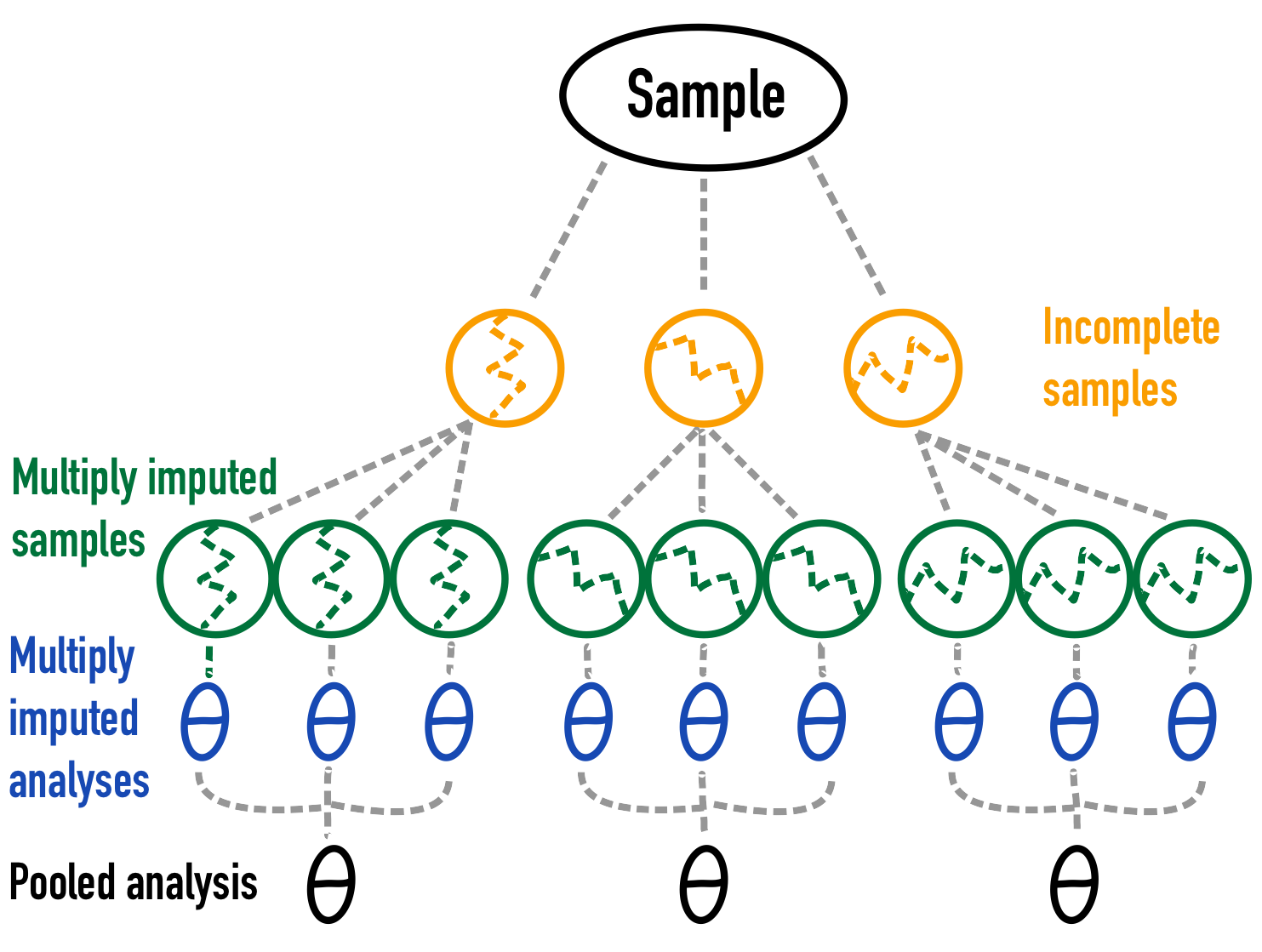
Instead of sampling data from a large data set or from a theoretical model, we can also take a single finite observed set as our comparative truth. With missing data simulations, this means that we can eliminate sampling variance from the evaluations of the imputation performance (Vink and van Buuren 2014).
Figure 4: A graphical depiction of missing data simulation with only missing data variance 3.
(Rubin 1987) defined \(Q\) as the quantity of interest (possibly a vector) and \(U\) as its variance. With multiple imputation, \(m\) complete data estimates can be averaged as \[\bar{Q}=\frac{1}{m}\sum^{m}_{l=1}{ \hat{Q}}_{l},\]
where \(\hat Q_l\) is an estimate of \(Q\) from the \(l\)-th imputed data set. Let \(\bar U_l\) be the estimated variance-covariance matrix of \(\hat Q_l\). The complete data variances of \(Q\) can be combined by
\[\bar{U}=\frac{1}{m}\sum^{m}_{l=1}{ {\bar U}}_{l}.\] The variance between the complete data estimates can be calculated as
\[B=\frac{1}{m-1}\sum^{m}_{l=1}(\hat{ Q}_l-\bar{Q})^\prime(\hat{ Q}_l-\bar{Q}).\]
The total variance of \(({ Q}-\bar{Q})\) is defined as
\[T=\bar{U}+B+B/m.\]
For populations for which all units are recorded, the average complete data variance \(\bar{U}\) of \(Q\) equals zero - there is no sampling variation - and the total variance of \(({Q}-\bar{Q})\) simplifies to
\[T=B+B/m.\] As a consequence, the relative increase in variance due to nonresponse equals \(r = (1+{m^{-1}}) B/\bar{U}= \infty\)4, and the degrees of freedom \(\nu\) can be set to
\[\nu = (m-1)(1+r^{-1})^2=m-1.\]
In simulation, we can make use of this property by taking a single finite complete set as our comparative truth and only induce missingness in it. The induced missingness would then serve as the necessary Monte Carlo variation.
Model-based finite populations
To demonstrate the validity of the above approach, we will draw a single finite set from the before used multivariate normal distribution:
truth <- mvtnorm::rmvnorm(n = 200,
                          sigma = sigma) %>%
  magrittr::set_colnames(c("x", "z")) %>% # add column names
  as_tibble() %>% # convert to tibble
  mutate(y = 6 * x + 3 * z + rnorm(200)) # add y
We perform the simulations as per our outlined simulation set-up, with the difference that our finite object truth now serves as the root of simulation and no sampling of cases is performed, other than the usual sampling of MCAR or right-tailed MAR missingness.
mbased_finite <- list(
  MCAR = furrr::future_map(1:1000, ~ { # map over 1000 sims
      truth %>%
        ampute(prop = .5,
               mech = "MCAR") %>% .$amp %>%
        mice(m = 5,
             maxit = 5,
             method = "norm",
             print = F)
    }, .options = furrr_options(seed = 123)),
  MAR = furrr::future_map(1:1000, ~ { # map over 1000 sims
      truth %>%
        ampute(prop = .5,
               mech = "MAR", type = "RIGHT") %>% .$amp %>%
        mice(m = 5,
             maxit = 5,
             method = "norm",
             print = F)
    }, .options = furrr_options(seed = 123))
)
We can evaluate the simulations by excluding the average sampling variance \(\bar{U}\) (ubar in mice) from the total variance calculations. First, we extract the true estimand from the finite set truth:
true <- truth %$%
  lm(y ~ x + z) %>%
  coefficients()
true
(Intercept) x z
0.008986397 6.112860965 2.965053625 Next, we evaluate the imputations agains truth:
mbased_finite %>%
  map(~.x %>% # for every missingness mechanism
    map(~.x %>% # for every simulated multiple imputation....
        complete("all") %>% # create a list of completed data sets
        map(~.x %$% # for every completed data set....
              lm(y ~ x + z) # fit linear model
        ) %>%
          pool(custom.t = ".data$b + .data$b / .data$m") %>% # pool coefficients
          .$pooled %>% # extract table of pooled coefficients
          mutate(true = true, # add true
                 df = m-1,  # correct df
                 riv = Inf, # correct riv
                 std.error = sqrt(t), # standard error
                 statistic = estimate / std.error, # test statistic
                 p.value = 2 * (pt(abs(statistic),
                                   pmax(df, 0.001),
                                   lower.tail = FALSE)), # correct p.value
                 `2.5 %` = estimate - qt(.975, df) * std.error, # lower bound CI
                 `97.5 %` = estimate + qt(.975, df) * std.error, # upper bound CI
                 cov = `2.5 %` < true & true < `97.5 %`, # coverage
                 bias = estimate - true) %>% # bias
          select(term, m, true, estimate, std.error, statistic, p.value,
                 riv, `2.5 %`, `97.5 %`, cov, bias) %>%
          column_to_rownames("term") # `term` as rownames
    ) %>%
      Reduce("+", .) / length(mbased_MCAR)
  )
Note that in the above code - despite the correct variance calculations - the following estimates needed manual adjustment: df, riv and p.value. The line pool(custom.t = ".data$b + .data$b / .data$m") ensures that the estimates, total variance, standard error and the test-statistic are correctly calculated. Since all other calculations depend on those estimates, a simple manual calculation of intervals and coverages suffices.
$MCAR
            m        true    estimate  std.error  statistic      p.value riv
(Intercept) 5 0.008986397 0.008326881 0.06546573  0.1420038 5.167269e-01 Inf
x           5 6.112860965 6.116552345 0.08745088 84.3572866 5.563203e-07 Inf
z           5 2.965053625 2.963656639 0.09098966 38.7037454 1.127899e-05 Inf
                 2.5 %    97.5 %   cov          bias
(Intercept) -0.1734351 0.1900889 0.956 -0.0006595154
x            5.8737498 6.3593549 0.948  0.0036913796
z            2.7110288 3.2162844 0.929 -0.0013969863

$MAR
            m        true     estimate  std.error  statistic      p.value riv
(Intercept) 5 0.008986397 -0.009431595 0.07060251 -0.1709634 4.897327e-01 Inf
x           5 6.112860965  6.082290519 0.09246685 77.9500305 6.603373e-07 Inf
z           5 2.965053625  2.991248281 0.09165275 39.0423374 1.179988e-05 Inf
                 2.5 %    97.5 %   cov        bias
(Intercept) -0.2054556 0.1865924 0.949 -0.01841799
x            5.8255614 6.3390197 0.958 -0.03057045
z            2.7367795 3.2457171 0.943  0.02619466
We can see that this adjusted variance simulation set-up yields valid inferences and allows for sharp comparisons between simulation scenarios and - if applicable - simulation methods.
Design-based finite populations
To demonstrate the validity of the finite population approach on design-based simulations, we will use one of the sampled sets from the design-based simulation section above.
which <- sample(1:length(simdata), 1)
truth <- simdata[[which]]
We perform the simulations as per our outlined simulation set-up, with the difference that our finite object truth now serves as the root of simulation and no sampling of cases is performed, other than the usual sampling of MCAR or right-tailed MAR missingness.
dbased_finite <- list(
  MCAR = furrr::future_map(1:1000, ~ { # map over 1000 sims
      truth %>%
        ampute(prop = .5,
               mech = "MCAR") %>% .$amp %>%
        mice(m = 5,
             maxit = 5,
             method = "norm",
             print = F)
    }, .options = furrr_options(seed = 123)),
  MAR = furrr::future_map(1:1000, ~ { # map over 1000 sims
      truth %>%
        ampute(prop = .5,
               mech = "MAR", type = "RIGHT") %>% .$amp %>%
        mice(m = 5,
             maxit = 5,
             method = "norm",
             print = F)
    }, .options = furrr_options(seed = 123))
)
We can evaluate the simulations by excluding the average sampling variance \(\bar{U}\) (ubar in mice) from the total variance calculations. First, we extract the true estimand from the finite set truth:
true <- truth %$%
  lm(y ~ x + z) %>%
  coefficients()
true
(Intercept) x z
0.319090 5.948874 3.015578 Next, we evaluate the imputations agains truth:
dbased_finite %>%
  map(~.x %>% # for every missingness mechanism
    map(~.x %>% # for every simulated multiple imputation....
        complete("all") %>% # create a list of completed data sets
        map(~.x %$% # for every completed data set....
              lm(y ~ x + z) # fit linear model
        ) %>%
          pool(custom.t = ".data$b + .data$b / .data$m") %>% # pool coefficients
          .$pooled %>% # extract table of pooled coefficients
          mutate(true = true, # add true
                 df = m-1,  # correct df
                 riv = Inf, # correct riv
                 std.error = sqrt(t), # standard error
                 statistic = estimate / std.error, # test statistic
                 p.value = 2 * (pt(abs(statistic),
                                   pmax(df, 0.001),
                                   lower.tail = FALSE)), # correct p.value
                 `2.5 %` = estimate - qt(.975, df) * std.error, # lower bound CI
                 `97.5 %` = estimate + qt(.975, df) * std.error, # upper bound CI
                 cov = `2.5 %` < true & true < `97.5 %`, # coverage
                 bias = estimate - true) %>% # bias
          select(term, m, true, estimate, std.error, statistic, p.value,
                 riv, `2.5 %`, `97.5 %`, cov, bias) %>%
          column_to_rownames("term") # `term` as rownames
    ) %>%
      Reduce("+", .) / length(mbased_MCAR)
  )
$MCAR
m true estimate std.error statistic p.value riv
(Intercept) 5 0.319090 0.3071532 0.27420289 1.318445 3.744276e-01 Inf
x 5 5.948874 5.9518494 0.04213763 169.069926 3.027307e-08 Inf
z 5 3.015578 3.0114404 0.03998183 90.585963 3.726015e-07 Inf
2.5 % 97.5 % cov bias
(Intercept) -0.4541561 1.068462 0.955 -0.011936856
x 5.8348566 6.068842 0.949 0.002975250
z 2.9004331 3.122448 0.957 -0.004137616
$MAR
m true estimate std.error statistic p.value riv
(Intercept) 5 0.319090 0.3848983 0.27095351 1.643707 3.126676e-01 Inf
x 5 5.948874 5.9398700 0.04256856 162.385704 3.015325e-08 Inf
z 5 3.015578 3.0167730 0.03944059 90.237449 3.364306e-07 Inf
2.5 % 97.5 % cov bias
(Intercept) -0.3673892 1.137186 0.956 0.065808335
x 5.8216807 6.058059 0.954 -0.009004194
z 2.9072684 3.126278 0.969 0.001195002We can see that this adjusted variance simulation set-up also yields valid inferences for design based simulations on a single finite set.
Conclusion
We have seen that it is straightforward to simulate missingness in R. Some of the outlined simulation scenarios may be more fitting to your aim or simulation set-up, but in all simulated cases there is the option to exclude the sampling of data sets and only sample the missingness. This may allow for a sharper comparison between imputation methods, as only the performance on solving for the missingness can impact method performance.
Please note that excluding sampling variance is not an option on real-life data sets, except for the scenario where all records from a real-life incomplete finite population are observed.
References
Session info
sessionInfo()R version 4.2.2 (2022-10-31)
Platform: aarch64-apple-darwin20 (64-bit)
Running under: macOS Monterey 12.6
Matrix products: default
BLAS: /Library/Frameworks/R.framework/Versions/4.2-arm64/Resources/lib/libRblas.0.dylib
LAPACK: /Library/Frameworks/R.framework/Versions/4.2-arm64/Resources/lib/libRlapack.dylib
locale:
[1] en_US.UTF-8/en_US.UTF-8/en_US.UTF-8/C/en_US.UTF-8/en_US.UTF-8
attached base packages:
[1] stats graphics grDevices utils datasets methods base
other attached packages:
[1] tibble_3.1.8 dplyr_1.0.10 magrittr_2.0.3 mvtnorm_1.1-3 furrr_0.3.0
[6] future_1.29.0 purrr_0.3.5 mice_3.15.0
loaded via a namespace (and not attached):
[1] Rcpp_1.0.9 pillar_1.8.1 compiler_4.2.2 tools_4.2.2
[5] digest_0.6.31 jsonlite_1.8.4 evaluate_0.15 lifecycle_1.0.3
[9] lattice_0.20-45 pkgconfig_2.0.3 rlang_1.0.6 cli_3.4.1
[13] DBI_1.1.2 rstudioapi_0.13 parallel_4.2.2 yaml_2.3.5
[17] xfun_0.31 fastmap_1.1.0 stringr_1.5.0 knitr_1.39
[21] globals_0.16.2 generics_0.1.3 vctrs_0.5.1 htmlwidgets_1.5.4
[25] grid_4.2.2 tidyselect_1.2.0 glue_1.6.2 listenv_0.8.0
[29] R6_2.5.1 parallelly_1.32.1 fansi_1.0.3 rmarkdown_2.14
[33] tidyr_1.2.1 codetools_0.2-18 backports_1.4.1 htmltools_0.5.4
[37] assertthat_0.2.1 utf8_1.2.2 stringi_1.7.8 broom_1.0.1 Footnotes
Note that for reasons of simplicity only the pooled analysis for 3 simulations and the multiply imputed samples for 3 imputations for each of those 3 simulations are shown. In real life this should be increased to obtain a more stable Monte Carlo simulation result.↩︎
Note that for reasons of simplicity only the pooled analysis for 3 simulations and the multiply imputed samples for 3 imputations for each of those 3 simulations are shown. In real life this should be increased to obtain a more stable Monte Carlo simulation result.↩︎
Note that for reasons of simplicity only the pooled analysis for 3 simulations and the multiply imputed samples for 3 imputations for each of those 3 simulations are shown. In real life this should be increased to obtain a more stable Monte Carlo simulation result.↩︎
I know!↩︎